basic statistics for data scientists PART 1
April 27, 2019
Introduction
The way I like to think of statistics is of two ways:
- Statistics for descriptive purposes
- Statistics for inference purposes
Descriptive Statistics
This helps the researcher understand the dataset that they have at hand. If the data at hand is for the entire population of interest, then plots like histograms, bar charts or summaries such as the mean and median will help one better understand the population. On the other hand, if the data at hand is a sample from the population then the same exact tools, plots and statistics, this time will help better understand the sample at hand. Bivariate plots can also be considered as descriptive statistics that shows you how the variables in your dataset behave together.
Descriptive statistics are essential since data is usually big and we need tools to summarize the information in them to understand it better.
In this post I will not focus on descriptive statistics as most data scientists are quite competent in making summary statistics and plots but it never hurts to emphasize the importance of looking at descriptives before starting an analysis.
Inferential Statistics
The fundamental difference that separates inferential statistics from descriptive statistics is the use of statistical theory to make inferences about the population of interest using only a sample from the said population.
Many use cases at tech companies, including but not limited to AB testing, are of this kind. In an AB test, we are not only interested in the visitors that arrive in an AB experiment but rather we want to use the information we gather from these visitors to understand our entire user base.
From this perspective all experiment data is sample data and AB tests and methods are mostly inferential to give the experimenter ideas about the users of the product, the population.
Definitions to Help with Inferential Statistics
Population: Population refers to the entire set of units that we want to learn about.
Parameter: Parameters refer to populations only. These are summaries about the population that may be of interest to us. By convention we label parameters with Greek letters. Again usually by convention \(\mu\) is reserved for population mean, \(\pi\) is reserved for population proportion and \(\Delta\) is reserved for the differences in two populations. We can use subscripts to further clarify \(\Delta\)s if need be like \(\Delta_{Mean}\) and \(\Delta_{Proportion}\) etc.
Sample: Sample in contrast is only a subset of the population. If we sample completely at random from the population, then the sample will have nice properties for inference. However, any subset of the population is a sample. As mentioned earlier, in relation to AB testing, experiment data is sample data that come from a bigger population of visitors that we want to generalize to.
Statistic: Summaries at the sample level are called statistics. So sample mean, sample median, sample proportion are all statistics. Statistics are labeled with Latin letters mostly. So \(\bar{X}\) for sample mean, \(p\) for sample proportion, and \(D\) for sample differences etc.
Sampling Distribution Sampling distribution is the key that opens the gateways from sample world to population world. Sampling distribution is what allows us to make inferences about the population parameters given sample statistics. So what is the sampling disribution?
Let’s imagine a case where the parameter of interest is the population mean. For a given sample size, if you were to collect all possible samples of this size and measured the means of these samples you would obtain as many means as there are samples. The distribution of all these means is called the sampling distribution.
Some Theory and An Example to Summarize All the Information So Far
- *Do I need to bootstrap to get the sampling distribution?
This is where statistical theory comes to our rescue. Even though bootstrapping by sampling with replacement from our original sample data and creating a sampling distribution this way sounds very intuitive to most data scientists, statistical theory allows us to get more certain results with less work.
Here are some results we utilize for AB testing to do inference
Theorem Let \(X_{1},...,X_{n}\) be a random sample from a population with mean \(\mu\) and variance \(\sigma^{2} < \inf\). Then
- \(E\bar{X} = \mu\)
- \(Var \bar{X} = \sigma^{2}/n\)
As long as the sample points in our sample come from independent and identically distributed random variables then theory tells us that the mean of the sampling distribution is the same as the true population mean and the variance of the sampling distributions equals the true variance in the population divided by our sample size.
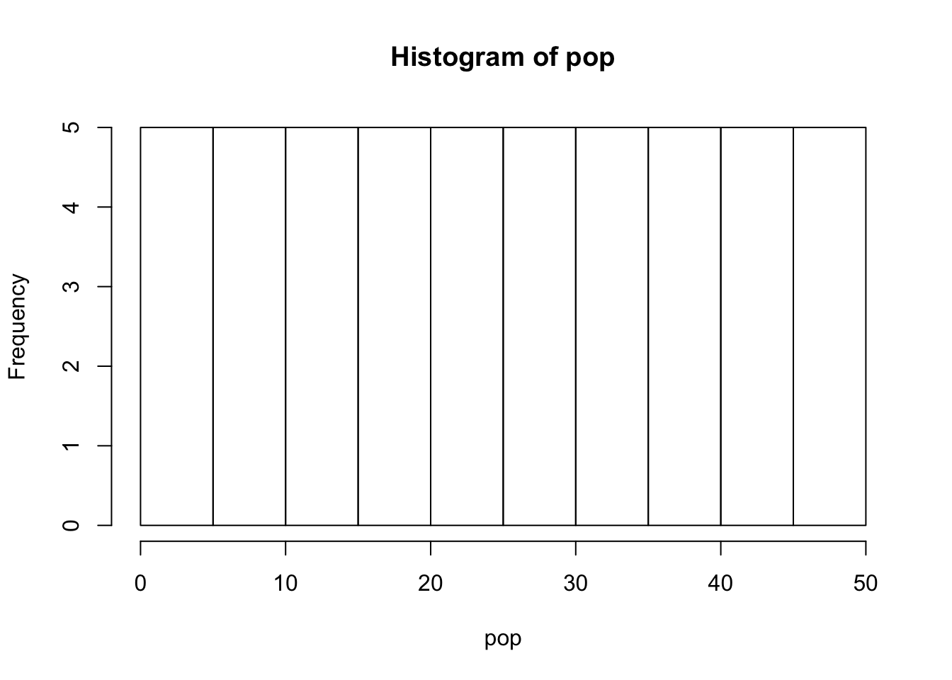
Imagine for argument’s sake that the population of interest consists of 50 data points only. \(\mathcal{P} = \{1,2,3,...,50\}\)

We are interested in the parameter, population mean \[ \mu = \frac{1+2+...+50}{50} = 25.5 \] The population variance is 208.25.
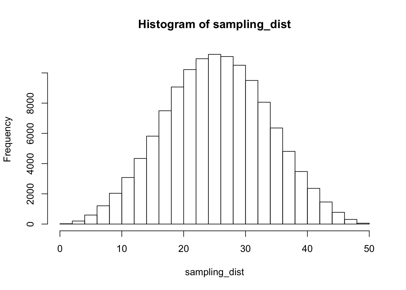
Let’s further say we take samples of size 3 from this population. Since we are sampling with replacement, the total number of samples we can get is \(50 \times 50 \times 50\). Let’s create a dataframe with all these samples and calculate the means for each to get the sampling distribution.
col1 <- rep(c(1:50), each = 2500)
col2 <- rep(rep(1:50, each = 50),50)
col3 <- rep(c(1:50), 250)

all_samples_with_replacement <- data.frame(X1 = col1, X2 = col2, X3 = col3)
sampling_dist <- rowMeans(all_samples_with_replacement)

nr_samples <- length(sampling_dist)

hist(sampling_dist)
exp_x_bar <- mean(sampling_dist)
sampling_var <- var(sampling_dist)*(nr_samples-1)/nr_samples

ifelse(identical(mu, exp_x_bar), 'The population mean equals the mean of the sampling distribution',
       'The population mean does not equal the mean of the sampling distribution')
## [1] "The population mean equals the mean of the sampling distribution"ifelse(identical(variance/3, sampling_var), 'The population variance divided by sample size equals the variance of the sampling distribution','The population variance divided by sample size does not equal the variance of the sampling distribution')## [1] "The population variance divided by sample size equals the variance of the sampling distribution"In a later post (Part 2), we will go over one-sample tests for the mean and proportion which then will allow us to extend those to two-sample tests, which are the tests commonly used in AB testing (base and variant being samples from two different populations).
These tests rely on the theory we have covered in this introductory chapter. We learned about the connection between the mean and variance of the sampling distribution and true mean and true variance in the population. One final piece we need is the shape of the sampling distribution. In the histrogram, it looked very much like a normal distribution. Was that a coincidence?
Central Limit Theorem
Central Limit Theorem (CLT) provides the last piece of the puzzle to go from samples to the population. It states
Let \(X_{1},...,X_{n}\) be a sequence of iid random variables whose moment generating functions exist in a neighborhood of 0. Let \(EX_{i} = \mu\) and \(Var X_{i} = \sigma^{2} > 0\) Define \(\bar{X_{n}} = (1/n) \sum_{i=1}^{n}X_{i}\). Let $G_{n}(x) denote the cdf of \(\sqrt{n}(\bar{X_{n}}-\,u)/\sigma\) Then, for any x, \(-\inf < x < \inf\), \[ lim_{n -> \inf}G_{n}(x) = \int_{-inf}^{x} \frac{1}{\sqrt{2\pi}}e^{-y^{2}/2}dy\]
All technicalities like finite and positive variances aside, what this theorem tells for us is that as the sample size increases, the sampling distribution of the mean will converge to a normal distribution.
How quickly this convergence happens, we do not know, it depends on the original population distribution, if the population itself is normally distributed, then we know the sampling distribution is normally distributed even with sample size = 1. When the popuplation distribution is not normally distributed, sampling distribution will converge to a normal eventually with increasing sample size.
for a more detailed analysis on the convergence to normality, see the link
This is a very usuful and powerful result because with the distributions shape, variance and mean known we can start calculating probabilities and quantify uncertainties around inferential estimates. In the next post, we will do exactly this.