Definitions

1. Null Hypothesis: This is the hypothesis we want to reject. So we assume this is true and then gather evidence against it to be able to reject it. If the evidence against the null at the end of an experiment is strong enough, by a measure of strength to be defined soon, we reject the null hypothesis.

2. Alternative Hypothesis: Alternative hypothesis is the negation of the null hypothesis. The union of the two should always cover all potential parameter values.

3. One-sided vs Two-sided tests: Tests whose null hypothesis are posed in the form of ‘parameter is less than/greater than a certain value’ are called one-sided tests while those whose null hypothesis is posed in the form of ‘parameter is equal to a certian value’ are called two-sided tests. All comparative tests (‘regular AB’), are two sample two sided tests. They test whether the difference between two populations is 0 or not. If the difference observed is too far away from 0 in either direction (improvement or hurting) we reject and can conclude the treatment is hurtful or benefitial. On the other hand, the non-inferiority test is a one-sided test. It tests whether the difference between two populations is less than the non-inferiority threshold or not. If we reject the null, we can conclude that the difference is not less than our allowed cost but we can never make a claim for results that are in the other direction.

4. Test-statistic: The test statistic is the standardized quantity of the observed statistic coming from the experiment. Put other way, the test statistic tells us how many standard deviations the observed statistic is away from the hypothesized mean. For example, if the statistic we collect is the sample mean, then the test statistic is the standardized observed mean. The test-statistic allows us to see where on the standardized sampling distribution our observation falls. Standardization allows us to communicate how extreme the observed quantity is regardless of the context (read units).

5. p-value: The p-value of a test is what quantifies the ‘strength’ of the evidence against the null. P-value is the probability that we would get a result that is as extreme or more as the one we observed if the null hypothesis is true. It translates to the area beyond the test statistic under the standardized sampling distribution.

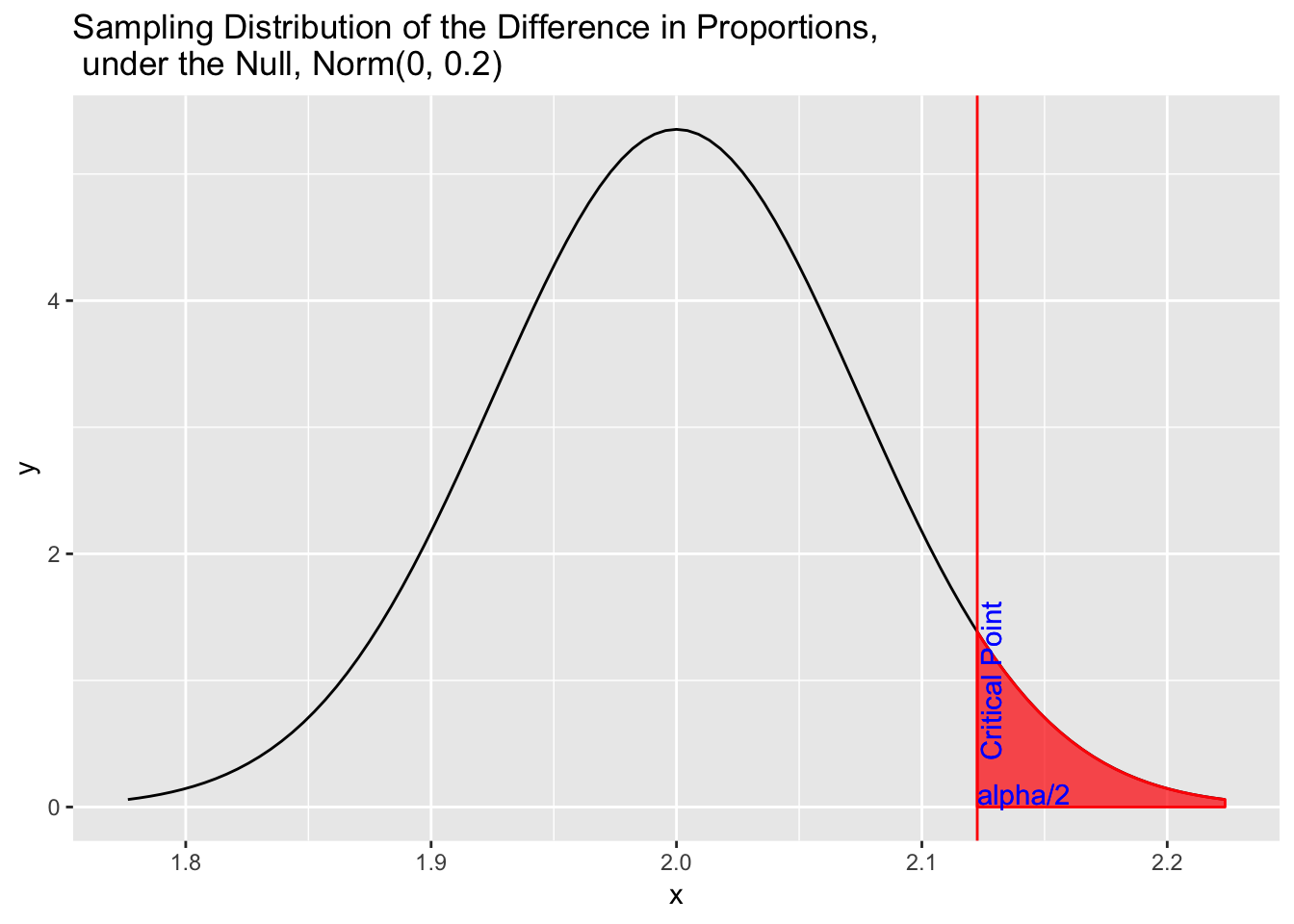
6. Critical Point and Rejection Region: The critical point is the point on the standardized sampling distribution beyond which we would reject the null hypothesis. Where this point lies depends on the false positive rate referred as \(\alpha\). In ET, we use \(\alpha = 0.10\) for comparative tests and an \(\alpha\) value of $0.10The area beyond the critical point is sometimes referred as the rejection region.

One Sample Test for the Mean

Let’s put all the definitions above to use with an example of a one-sample test for the mean.

Consider the case where we want to know whether the mean page load time is greater than 2 miliseconds.

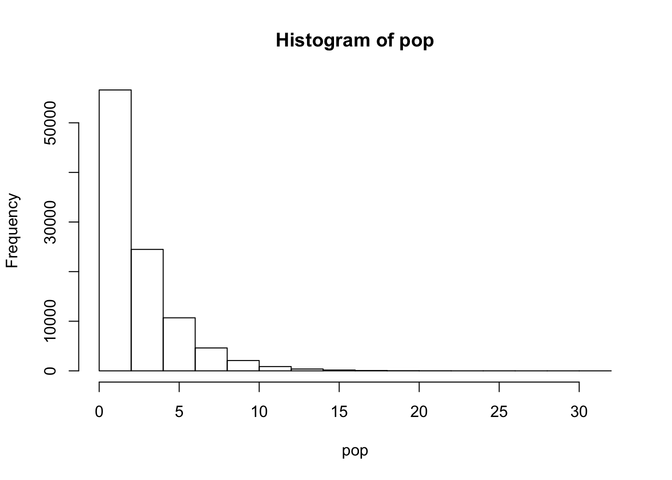
\[ H_{0}: \mu <= 2 \text{ms} \] \[ H_{1}: \mu > 2 \text{ms} \] Let’s say for arguments sake we have access to the entire population and the population has a mean of 2.4ms pageload time that is coming from an exponential distribution (to make the point that a normally distributed population is not required).

set.seed(7)

N <- 100000
pop <- rexp(N, 1/2.4)
mu <- mean(pop)
sigma <- sqrt(var(pop)*(N-1)/N)
hist(pop)

n <- 1000
samp <- sample(x = pop,size =  n, replace = FALSE)
x_bar <- mean(samp)
sigma_hat <- sqrt(var(samp))


se <- sqrt((sigma_hat^2)/n)

t.test(samp, mu = 2, alternative = 'greater')

## 
##  One Sample t-test
## 
## data:  samp
## t = 3.2782, df = 999, p-value = 0.0005403
## alternative hypothesis: true mean is greater than 2
## 95 percent confidence interval:
##  2.121613      Inf
## sample estimates:
## mean of x 
##  2.244309

Let’s put all the things we covered in previous chapter to use.

Assuming the null hypothesis is correct, the mean of the sampling distribution will be centered at the true mean which is 2ms. The standard deviation of the sampling distribution (standard error from now on) will be the true population variance divided by the sample size (\(\sigma^{2}/N)\)), and therefore

\(\frac{\bar{X} - \mu}{\sqrt{\sigma^{2}/N}} \sim N(0,1)\). However, note that to leverage this information, we need to know the true population variance \(\sigma^{2}\). If we use our sample to estimate this parameter \(\hat{\sigma}^{2}\) theory tell us \(\frac{\bar{X} - \mu}{\sqrt{\hat{\sigma}^{2}/N}} \sim T(0,df=N-1)\).

Then, if the null is true,

\(\frac{\bar{X} - \mu}{\sqrt{\hat{\sigma}^{2}/N}} \sim T(0,df=N-1)\)

which means, if \(H_{0}\) is true 3.2782255 is a draw from \(T(0,df=1000-1)\)

the critical value is 1.6463803. Since our test statistic is greater than the critical value, meaning what we observed is more extreme than what we subjectively allow to be attributable to chance (5%), we will reject the null and conclude that the average pageload time is greater than 2ms.

One Sample Test for Proportions

In this example, we will compare proportions intead of means of continuos variables.

Consider the case where we want to know whether the conversion on a certain page for a certain metric is 0.5 or not.

\[ H_{0}: \pi = 0.5 \] \[ H_{1}: \pi \neq 0.5 \]

set.seed(7)

N <- 100000
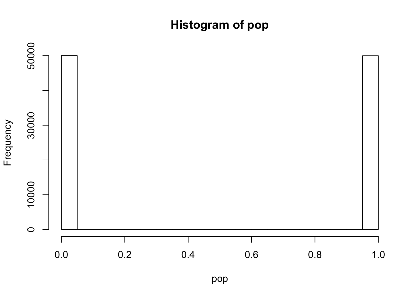
pop <- rbinom(n = N, size = 1, p = 0.5)
pi <- mean(pop)
sigma <- sqrt(var(pop)*(N-1)/N)
sigma2 <- sqrt(pi*(1-pi))
hist(pop)

n <- 1000
samp <- sample(x = pop,size =  n, replace = FALSE)
p <- mean(samp)

If the null hypothesis is correct, we know that

\[ \frac{p - \pi}{\sqrt{\sigma^{2}/N}} \sim N(0,1) \] The difference of proportions from means is that we do not need to estimate \(\sigma\) because there is a direct relationship between mean and variance for a binomial distribution. That is,

\[ \sigma^{2} = \pi * (1- \pi) \]. So, \[ \frac{p - \pi}{\sqrt{\pi (1-\pi)/N}} \sim N(0,1) \]

This is so, as long as the distribution of proportion can be approximated with a normal distribution. But we know normal approximation for a binomial distribution is a good one so long as the sample size is not too small.

Then under \(H_{0}\), we expect 1.2649111 to be N(0,1).

So, our observed proportion is 1.2649111 standard deviation away from zero. We will reject the null if the observed proportion is at least 1.6448536 standard deviations away from zero. Since 1.2649111 isn’t greater than 1.6448536 we fail to reject the null hypothesis.

The p-value is 1.7940968 which is not less than 0.05, another way of looking at whether the result is significant or not.

the test we have conducted above is known as a one sample z-test.

The G-Test, The Chi-Squared Test and Their Connection to the z-test in ET

You may have heard that AB tests use a G-test for binary metrics and not the z-test. Is there a difference? Let us start with a Chi Squared test. We will show that for a binary metric, a z-test and a Chi-Squared test are equavalent and then make the connection between the chi squared test and the G test. Again most AB test platforms use the G-test to test binary metrics.

We can represent our data as total number of 1s and 0s (1 = converted, 0 = did not convert).

If the null is correct and \(\pi = 0.5\), then we expect 500 converters and 500 non converters.

library(knitr)
library(tidyverse)

## ── Attaching packages ──────────────────────────────────────────────────────────────────────────────────────────────────────── tidyverse 1.2.1 ──

## ✔ ggplot2 3.1.0     ✔ purrr   0.2.5
## ✔ tibble  2.0.0     ✔ dplyr   0.7.8
## ✔ tidyr   0.8.2     ✔ stringr 1.3.1
## ✔ readr   1.3.1     ✔ forcats 0.3.0

## ── Conflicts ─────────────────────────────────────────────────────────────────────────────────────────────────────────── tidyverse_conflicts() ──
## ✖ dplyr::filter() masks stats::filter()
## ✖ dplyr::lag()    masks stats::lag()

summ <- as.tibble(table(samp))

## Warning: `as.tibble()` is deprecated, use `as_tibble()` (but mind the new semantics).
## This warning is displayed once per session.

summ <- summ %>% 
  transmute(Cell = samp,
            Observed = n) %>% 
   mutate(Expected = c(500,500))

kable(summ)

The chi squared goodness of fit test then says:

\[ \sum_{i=1}^{C} \frac{(O_{i}-E_{i})^2}{E_{i}} \sim \chi_{k} \]

where i is an index for cells, N is the total number of cells and k is the degrees of freedom for the chi squared distribution.

In a binary metric case, C = 2, and k = C - 1 = 1.

If the hypothesized proportion of map bookers is \(\pi\) and observed proportion is \(p\) realize

\[O_{1} = Np \text{ and } O_{2} = N - Np = N (1-p)\] \[E_{1} = N \pi \text{ and } E_{2} = N - N \pi = N(1-\pi)\] Plugging the above into the test statistic we get:

\[ \frac{(Np - N \pi)^{2}}{N \pi} + \frac{\bigg(N\big((1-p)-(1-\pi)\big)\bigg)^2}{N(1-\pi)}\]

A little algebra gets us:

\[ \bigg(\frac{(p - \pi)}{\sqrt{(\pi(1-\pi)/N)}}\bigg)^{2} \]

Observe the test statistic for the chi-square test for a binomial metric is the test statistic we used in the z test raised to second power. So we expect it to be distributed as the square of a standard normal. And a chi-square distribution with one degree of freedom is defined to be the square of a standard normal.

So testing the square of the test ststistic using a chi square distribution with 1 degree of freedom is equivalant to testing the test statistic using a standard normal.

To see this real quick, if we look at the p-value for the chi-square test we will see where on a chi-square (df=1) distribution the test statistic squared falls. 0.2059032. Realize we get the same p-value as the z-test.

Okay now that we have established the equavalance between the z and chi square tests for binary metrics, let’s finally go over the G-test.

G-test is what is known a likelihood ratio test. The test statistic is

\[ G = 2 \sum_{i=1}^{C}O_{i} \text{ ln}\big(\frac{O_{i}}{E_{i}}\big) \] G is approximately distributed as a chi-square with C - 1 degrees of freedom like the chi-square test statistic. Asymptotically G like Chi square test statistic is chi-square distributed.

Confidence Intervals and p-value CI duality

library(ggplot2)
p <- ggplot(data.frame(x = c(2 - 0.07452485*3, 2 + 0.07452485*3)), aes(x)) + 
  stat_function(fun = dnorm, args = list(mean = 2, sd = 0.07452485)) +
  stat_function(fun = dnorm, args = list(mean = 2, sd = 0.07452485), xlim = c(qnorm(.1/2,2,0.07452485,FALSE), 2 + 0.07452485*3), geom = "area", fill='red', color='red', alpha = 0.7) 

p + geom_vline(xintercept=qnorm(.1/2,2,0.07452485,FALSE), color='red') +
    geom_text(aes(x=qnorm(.1/2,2,0.07452485,FALSE), label="Critical Point", y=1), colour="blue", angle=90, vjust = 1.2) +
    geom_text(aes(x=qnorm(.1/2,2,0.07452485,FALSE), label="alpha/2", y=0.1), colour="blue", hjust = 0, angle=0) + 
  ggtitle("Sampling Distribution of the Difference in Proportions, \n under the Null, Norm(0, 0.2)")